Day 3

Where do things live?

Working Directory

  • Directory where R first looks for files.
    • If you run read.csv("mydata.csv") then mydata.csv should be in your working directory
  • Check current location (your location will be different):
> getwd()
[1] "C:/Users/mgelman/Dropbox/econ122-f19/docs"
  • R Markdown: When you knit a .Rmd file, the working directory for the compilation of the document is always the directory where the .Rmd file is located!
    • This may be different from the location of your current Rstudio session.

Where do things live?

Workspace

  • This is the “environment” where R objects live.
    • See the Environment tab in Rstudio
  • Check the contents of my (or your) environment
> ls()
character(0)

(If it says character(0) then your workspace is empty!)

  • R Markdown: When you knit a .Rmd file, a completely new and separate working space is created.
    • why do you think this is the case?
    • R chunk may throw an error if you reference an object loaded in your workspace but not via R chunk

Where do things live?

Rstudio Projects

  • Projects set your working directory to the folder it lives in
    • easy way to set your working directory
    • can save and reload your workspace (environment)
  • Projects can be connected to GitHub using Rstudio’s GUI
  • Highly recommend: create a project for this class in the folder you are using to store class work.

Objects in R

  • Anything created or imported into R is called an object
    • vectors, data frames, matrices, lists, functions, lm, …
  • We usually store objects in the workspace using the assignment operator <-
> x <- c(8,2,1,3)
> ls()
[1] "x"
  • The = operator also does assignment, but it is mainly used for argument specification inside a function.
> y <- rnorm(3, mean=10, sd=2)
> ls()
[1] "x" "y"
  • Please don’t use = for variable assignment!!!

Data structures and types

Shape and computer storage

Data types

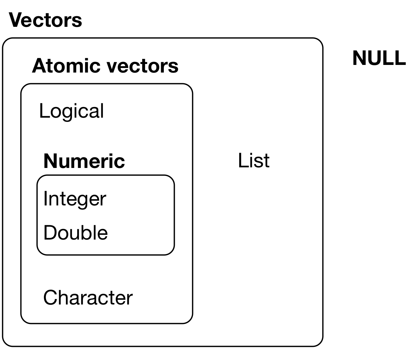
Determines computer storage of info

  • Important data types
    • Logical: TRUE and FALSE are the only values
    • Numeric class: Integer and double
    • Character: string ("") of text
> typeof(x)  # type of storage mode 
[1] "double"
> class(x)   # object class is numeric
[1] "numeric"
> typeof("abc")
[1] "character"
> x == 1
[1] FALSE FALSE  TRUE FALSE
> typeof(x == 1)
[1] "logical"

Vectors

Shape of an object

  • R uses two types of vectors to store info
    • atomic vectors: all entries have the same data type
    • lists: entries can contain other objects that can differ in data type
  • All vectors have a length
> x
[1] 8 2 1 3
> length(x)
[1] 4
> x.list<- list(x,1,"a")
> length(x.list)
[1] 3

Atomic Vectors: Matrices

  • You can add attributes, such as dimension, to vectors
  • A matrix is a 2-dimensional vector containing entries of the same type
> x
[1] 8 2 1 3
> x.mat <- matrix(x, nrow=2, byrow=TRUE)
> x.mat
     [,1] [,2]
[1,]    8    2
[2,]    1    3
> class(x.mat)
[1] "matrix"
> str(x.mat)
 num [1:2, 1:2] 8 1 2 3

Atomic Vectors: Matrices

  • or you can bind vectors of the same length to create columns or rows:
> x.mat2 <- cbind(x,2*x)
> x.mat2
     x   
[1,] 8 16
[2,] 2  4
[3,] 1  2
[4,] 3  6

Lists: Data frames

  • A data frame is a list of atomic vectors of the same length, but not necessarily the same data type
  • the loans data frame has columns that are integer and factor types
> loans <- read.csv("https://raw.githubusercontent.com/mgelman/data/master/CreditData.csv")
> class(loans)
[1] "data.frame"
> typeof(loans)
[1] "list"
> str(loans)
'data.frame':   1000 obs. of  21 variables:
 $ Status.of.existing.checking.account                     : Factor w/ 4 levels "... < 0 DM","... >= 200 DM / salary assignments for at least 1 year",..: 1 3 4 1 1 4 4 3 4 3 ...
 $ Duration.in.month                                       : int  6 48 12 42 24 36 24 36 12 30 ...
 $ Credit.history                                          : Factor w/ 5 levels "all credits at this bank paid back duly",..: 2 4 2 4 3 4 4 4 4 2 ...
 $ Purpose                                                 : Factor w/ 10 levels "business","car (new)",..: 8 8 5 6 2 5 6 3 8 2 ...
 $ Credit.amount                                           : int  1169 5951 2096 7882 4870 9055 2835 6948 3059 5234 ...
 $ Savings.account.bonds                                   : Factor w/ 5 levels ".. >= 1000 DM",..: 5 2 2 2 2 5 4 2 1 2 ...
 $ Present.employment.since                                : Factor w/ 5 levels ".. >= 7 years",..: 1 3 4 4 3 3 1 3 4 5 ...
 $ Installment.rate.in.percentage.of.disposable.income     : int  4 2 2 2 3 2 3 2 2 4 ...
 $ Personal.status.and.sex                                 : Factor w/ 4 levels "female : divorced/separated/married",..: 4 1 4 4 4 4 4 4 2 3 ...
 $ Other.debtors.guarantors                                : Factor w/ 3 levels "co-applicant",..: 3 3 3 2 3 3 3 3 3 3 ...
 $ Present.residence.since                                 : int  4 2 3 4 4 4 4 2 4 2 ...
 $ Property                                                : Factor w/ 4 levels "if not A121 : building society savings agreement/life insurance",..: 3 3 3 1 4 4 1 2 3 2 ...
 $ Age.in.years                                            : int  67 22 49 45 53 35 53 35 61 28 ...
 $ Other.installment.plans                                 : Factor w/ 3 levels "bank","none",..: 2 2 2 2 2 2 2 2 2 2 ...
 $ Housing                                                 : Factor w/ 3 levels "for free","own",..: 2 2 2 1 1 1 2 3 2 2 ...
 $ Number.of.existing.credits.at.this.bank                 : int  2 1 1 1 2 1 1 1 1 2 ...
 $ Job                                                     : Factor w/ 4 levels "management/ self-employed/highly qualified employee/ officer",..: 2 2 4 2 2 4 2 1 4 1 ...
 $ Number.of.people.being.liable.to.provide.maintenance.for: int  1 1 2 2 2 2 1 1 1 1 ...
 $ Telephone                                               : Factor w/ 2 levels "none","yes, registered under the customers name": 2 1 1 1 1 2 1 2 1 1 ...
 $ foreign.worker                                          : Factor w/ 2 levels "no","yes": 2 2 2 2 2 2 2 2 2 2 ...
 $ Good.Loan                                               : Factor w/ 2 levels "BadLoan","GoodLoan": 2 1 2 2 1 2 2 2 2 1 ...
Lists: Data frames

  • data frame attributes include column names and row.names
  • you can create a data frame with the data.frame command
> x.df <- data.frame(x=x,double.x=x*2)
> x.df
  x double.x
1 8       16
2 2        4
3 1        2
4 3        6
> attributes(x.df)  # note: attributes returns a list!
$names
[1] "x"        "double.x"

$class
[1] "data.frame"

$row.names
[1] 1 2 3 4

Data types: factors

  • Factors are a data type stored as integers
    • The attribute levels is a character vector of possible values
    • Values are stored as the integers (1=first level, 2=second level, etc)
> class(loans$Good.Loan)
[1] "factor"
> typeof(loans$Good.Loan)
[1] "integer"
> levels(loans$Good.Loan)
[1] "BadLoan"  "GoodLoan"
> str(loans$Good.Loan)
 Factor w/ 2 levels "BadLoan","GoodLoan": 2 1 2 2 1 2 2 2 2 1 ...
> head(loans$Good.Loan)
[1] GoodLoan BadLoan  GoodLoan GoodLoan BadLoan  GoodLoan
Levels: BadLoan GoodLoan

Object Oriented Programming

  • In R, commands care about object class and type
  • Ex: For a factor, what type of summary would be helpful?
> summary(loans$Good.Loan)
 BadLoan GoodLoan 
     300      700 
  • What about for a numeric?
> summary(loans$Duration.in.month)
   Min. 1st Qu.  Median    Mean 3rd Qu.    Max. 
    4.0    12.0    18.0    20.9    24.0    72.0 
  • In your Console window, type ?summary then hit tab.
    • see summary.default, summary.factor, …

Coercion

  • Entries in atomic vectors must be the same data type
  • R will default to the most complex data type if more than one type is given
> y <- c(1,2,"a")
> y
[1] "1" "2" "a"
> typeof(y)
[1] "character"

Coercion

  • Logical values coerced into 0 for FALSE and 1 for TRUE
> z <- c(TRUE, FALSE, TRUE, 7)
> z   # TRUE = 1, FALSE = 0
[1] 1 0 1 7
> typeof(z)
[1] "double"
  • Logical vectors are also coerced into numeric when applying math functions
> x
[1] 8 2 1 3
> x >= 5  # which entries >= 5?
[1]  TRUE FALSE FALSE FALSE
> sum(x >= 5)  # how many >=5 ?
[1] 1
> mean(x >= 5) # proportion of entries >=5
[1] 0.25

Subsetting: Atomic Vector

  • subset with [] by referencing index value (from 1 to vector length):
> x
[1] 8 2 1 3
> x[c(4,2)]  # get 4th and 2nd entries
[1] 3 2
  • subset by omitting entries
> x[-c(4,2)]  # omit 4th and 2nd entries
[1] 8 1
  • subset with a logical vector
> x[c(TRUE,FALSE,TRUE,FALSE)]  # get 1st and 3rd entries
[1] 8 1

Subsetting: Matrices

  • access entries using subsetting [row,column]
> x.mat2
     x   
[1,] 8 16
[2,] 2  4
[3,] 1  2
[4,] 3  6
> x.mat2[,1] # first column
[1] 8 2 1 3
> x.mat2[1:2,1] # first 2 rows of first column
[1] 8 2
  • R doesn’t always preserve class:
> class(x.mat2[1,])  # one row (or col) is no longer a matrix (1D)
[1] "numeric"

Subsetting: Data frames

  • you can access entries like a matrix:
> x.df
  x double.x
1 8       16
2 2        4
3 1        2
4 3        6
> x.df[,1]  # first column, all rows
[1] 8 2 1 3
> class(x.df[,1])  # first column is no longer a data frame
[1] "numeric"
  • One column of a data frame is no longer a data frame

Subsetting: Data frames

  • but one row with 2 or more columns (variables) is still a data frame
> x.df[1, 1:2]  # 1 row, 2 columns
  x double.x
1 8       16
> class(x.df[1, 1:2])
[1] "data.frame"
  • Remember that data frames are built from lists of variables (vectors) so they are different objects than matrices

Subsetting: Data frames

  • or access columns with $
> x.df$x  # get variable x column
[1] 8 2 1 3
  • you can also use column names to subset:
> loans[1:2,c("Good.Loan","Credit.amount")] # get 2 rows of Good.Loan and Credit.amount
  Good.Loan Credit.amount
1  GoodLoan          1169
2   BadLoan          5951

Subsetting: Lists

  • Recall: a list is a vector with entries that can be different object types
> my.list <- list(myVec=x, myDf=x.df, myString=c("hi","bye"))
> my.list
$myVec
[1] 8 2 1 3

$myDf
  x double.x
1 8       16
2 2        4
3 1        2
4 3        6

$myString
[1] "hi"  "bye"

Subsetting: Lists

  • one [] operator gives you the object at the given location but preserves the list type
  • my.list[2] return a list of length one with entry myDf
> my.list[2]
$myDf
  x double.x
1 8       16
2 2        4
3 1        2
4 3        6
> str(my.list[2])
List of 1
 $ myDf:'data.frame':   4 obs. of  2 variables:
  ..$ x       : num [1:4] 8 2 1 3
  ..$ double.x: num [1:4] 16 4 2 6

Subsetting: Lists

  • the double [[]] operator gives you the object stored at that location
    • can enter location number or entry name
  • my.list[[2]] or my.list[["myDf"]] return the data frame myDf
> my.list[[2]]
  x double.x
1 8       16
2 2        4
3 1        2
4 3        6
> str(my.list[[2]])
'data.frame':   4 obs. of  2 variables:
 $ x       : num  8 2 1 3
 $ double.x: num  16 4 2 6
> my.list[["myDf"]]
  x double.x
1 8       16
2 2        4
3 1        2
4 3        6

Subsetting: Lists

  • Like a data frame, can use the $ to access objects stored in the list
    • equivalent to using [[]]
  • my.list$myDf return the data frame myDf
> my.list$myDf
  x double.x
1 8       16
2 2        4
3 1        2
4 3        6
> class(my.list$myDf)
[1] "data.frame"

Functions

  • a function takes in objects and arguments and produces a new object
  • here are the various types of mean functions in R: (can depend on packages loaded)
> methods(mean)
[1] mean.Date     mean.default  mean.difftime mean.POSIXct  mean.POSIXlt 
see '?methods' for accessing help and source code

Functions

  • the default mean function code is here:
> mean.default
function (x, trim = 0, na.rm = FALSE, ...) 
{
    if (!is.numeric(x) && !is.complex(x) && !is.logical(x)) {
        warning("argument is not numeric or logical: returning NA")
        return(NA_real_)
    }
    if (na.rm) 
        x <- x[!is.na(x)]
    if (!is.numeric(trim) || length(trim) != 1L) 
        stop("'trim' must be numeric of length one")
    n <- length(x)
    if (trim > 0 && n) {
        if (is.complex(x)) 
            stop("trimmed means are not defined for complex data")
        if (anyNA(x)) 
            return(NA_real_)
        if (trim >= 0.5) 
            return(stats::median(x, na.rm = FALSE))
        lo <- floor(n * trim) + 1
        hi <- n + 1 - lo
        x <- sort.int(x, partial = unique(c(lo, hi)))[lo:hi]
    }
    .Internal(mean(x))
}
<bytecode: 0x0000000038d12b70>
<environment: namespace:base>

Functions

  • Function creation is not something we will emphasize in this Data Science course, but you should be able to create simple functions
my.function <- function(arguments)
{
  code that does the work
  
  return(list(objects that you are returning))
}
  • If you are returning only one object, you don’t need the list function in return

Functions

  • This function returns the mean and SD of a vector and (possibly) creates a histogram
    • input: variable x, plotting argument (default is FALSE)
    • …: optional arguments that might be used in mean and sd
    • output: list of mean and sd
> MeanSD <- function(x,plot=FALSE,...)
+ {
+   mean.x <- mean(x,...)
+   sd.x <- sd(x,...)
+   if (plot) 
+     hist(x)
+   return(list(Mean=mean.x,SD=sd.x))
+ }

Functions

  • A simple example:
> MeanSD(loans$Credit.amount)
$Mean
[1] 3271.258

$SD
[1] 2822.737
  • Function output is a list:
> str(MeanSD(loans$Credit.amount))
List of 2
 $ Mean: num 3271
 $ SD  : num 2823

Functions

Add plotting argument:

> MeanSD(loans$Credit.amount, plot=TRUE)

$Mean
[1] 3271.258

$SD
[1] 2822.737